Tuesday, July 4, 2017

Localization with a range finder

Discrete localization demo part 5


Localization via a range finder

In our last experiment, we simulated a robot with three color sensors pointed in different directions. In each of the tests, the robot easily localized itself. But in most robotics applications, robots often have distance data to its surroundings, instead of color information. We see this in simple robots that use ultrasonic range finders to detect walls and nearby objects. We also see this in complex platforms, e.g., self-driving cars often have rotating LIDAR(s) on top of the vehicle. This system maps the immediate neighborhood around the robot car. The LIDAR data output is typically a point cloud, indicating different points in the environment and their distances from the LIDAR. We will explore this range-based mechanism in a simplified simulation.

Simulation setup

We will not recreate a continuous point cloud. Instead, we will simply replace the color data from the three sensors in the previous post with distance information. We will also simplify the problem by assuming that a diagonal distance between cells is equal to the lateral or vertical distance between cells. This assumption is not an issue as long as the method of measurements is consistent when pre-storing map information and while navigating.

To show the changes in the distance data, we will make a slight change in the graph. We now put the location of the robot and the objects cells detected by the range finder in the first graph (upper left), and place the probability estimates on the lower right graph. The lower left remains the same, the map of the environment and the robot. On the upper right, we introduce a new graph where we plot (via a histogram) the detected distances for each of the three

Simulations

Our simulations will involve two runs, the first with 1 object type and the second with 2 object types. In theory, there should not be any difference in the localization between 1-object or 2-object runs since the range finder sensors cannot distinguish the object type, only its distance to the sensor. We will also test a low and high object density scenarios.

Low density runs


High density runs


We notice that the localization is not very precise and take many more iterations to reach a high-contrast prediction. This is expected. The number of distance possibilities that might match (or be a close match) to the current location is higher. In comparison, the very specific object type identity (via the color sensors) allows the algorithm to eliminate many cell locations as highly improbable. In a distance calculation, many more cell locations are likely locations, hence the spread out probabilities and lack of color contrast (compared to our previous simulations).

Improving the cell elimination

The problem with the above approach is that the many cells have distance calculation that are at least close to the distance measured by the range finders. Thus, they tend to maintain high probabilities as a potential robot location. One possible way to sharpen the guessing is to eliminate distance calculations that are less than a threshold away from the reported distance. This should quickly eliminate locations that are marginally viable. Let’s try this:

Low density runs


High density runs


Voila! We are able to quickly zoom in to the cells that are likely robot locations far quickly and with more contrast to neighboring cells.

Sunday, July 2, 2017

Localization via landmarks

Discrete localization demo part 4


Localization via landmarks

Our previous simulated robots have color sensors aimed down to detect the color of their current location in a map. Let’s show one that has color sensors aimed horizontally, to show a more realistic camera orientation. Our localization algorithm will therefore navigate using objects it encounters as localization landmarks.

Simulation setup

Let’s define our simulation parameters. For the most part, we will retain the modeling behavior from previous simulations, with some minor modifications.

Gridmap

We retain the same mechanics as before. The robot can move in any of four directions: left, right, up, and down. The robot has no heading orientation, so when it moves sideways, it does not rotate first. It simply moves sideways. The robot motion could be noisy, which means in some very rare instances, the robot might move diagonally. This is unlikely however. Its occurrence does not materially change the simulation. The robot moves over a cyclic gridmap, with each side continuing to the opposing edge. The gridmap is randomly populated with objects or structures.

Color sensors

We will design three color sensors that can read color at any distance with some accuracy. The sensor’s accuracy can change (can be modeled as less than perfect, as in previous simulations), but its accuracy remains the same over any distance. This is not a realistic representation --sensor accuracy, particularly color detection, weakens the farther the object being observed-- but good enough to show how localization in this manner would work. Changing the code to accommodate increasing sensor error with increasing distance is not hard, but unnecessary for a proof-of-concept. These sensors are fixed. They do not rotate when the robot changes direction.

Color sensor readout

The colors in each cell represent the color of the object/structure in that cell location (an object cell). The only exception is the color ‘green’, which we will use to denote ground, i.e., a ground cell and not a structure. The robot has three cameras, or color sensors: one aimed directly forward, one to the left at a 45 degree angle, and another one aimed 45 degrees to the right. Each sensor will detect the color of the first structure in its line-of-sight. Since ground is not at eye/sensor-level, the color sensors do not ‘see’ the green ground cells in its view path. The robot will detect the first non-ground structure, keeping in mind the cyclic nature of the gridmap. The structures detected by the three sensors are shown in the lower-right diagram during each iteration. For ease of coding, the robot can occupy the same cell as these objects (no collision detection).

Sensor diagram

On this diagram, the current robot location is identified as the ‘green’ cell. On a non-cyclic map, there should not be any highlighted cell below the current robot location, since all sensors are aimed up/forward. In our cyclic map, if the diagram shows a cell below the current robot location, it means one of the three sensors did not see a structure within the gridmap, and had to cycle through the opposing edge until it found a structure cell. We only cycle the sensor by one map width. If the sensor does not detect a structure after one cycle, the sensor reports ‘green’, the ground color. [This default color value is unnecessary, but I had to part the reading on some value.] Note that the robot has no information about how far these structures are relative to the robot. All the robot receives are three color information, one for each color sensor.

Simulations

Let’s run some simulations, varying the number of object types (number of different cell colors) and object density (total number of all objects in the gridmap).

1-object world

Let’s start with a world with only one type of object. We expect that this would take a little bit of time to localize. That said, a world with only one object type (two, including the ground cell) would be even more difficult to localize in our previous experiments with the single downward-looking color sensor. Intuitively, we would guess that the three-sensor model would work faster since it would eliminate more locations per iteration. We won't test this comparison however.


2-object world

Let’s do the same with a 2-object world, using roughly the same object density.


8-object world

Finally, let’s populate the robot world with eight types of objects, again maintaing approximately the same object density over the gridmap.


Low object-density world

We are also interested in localizing over a world where there are few landmarks. Let's repeat the above experiments, but with far fewer objects present.

1-object world

Let’s start with the 1-object test:


2-object world

Followed by the 2-object run:


8-object world

Finally, an 8-object low density test:


Closing thoughts

We showed a simplified model of a robot that uses cameras to detect objects, and use this information to localize itself. While the camera detection is crude --representing an object with a single color, assuming the camera only 'sees' one object at a time and does not model an expanding line-of-sight, accuracy at any distance is the same-- the mechanics remain applicable to a real-world application. Instead of identifying a color, an object or scene recognition system can process the camera stream and match the result to the map. Multiple cameras can add additional visual references to orient and localize a real robot.

In our next experiment, we will replace the color sensor with a distance sensor. Most navigation robots use a range finder to map its surroundings. Understanding visual cues and recognizing objects are still unreliable. Computer vision is hard, and processing images to generate a map is fundamentally more difficult than receiving raw distance data from a range finder. There is practically zero computing overhead with these sensors, and even cheap ultrasonic sensors have sufficient accuracy for simple applications. So it is time we model such a setup.

Sunday, June 25, 2017

Localization over heterogeneous features, part 2

Discrete localization demo part 3


Localization under different environments, part 2

This is a continuation of the previous post on localization under heterogenous features (see here), where we made clear that localization appears faster with more distinctive features present in an environment. The assumption of course is that the robot sensor is capable of distinguishing all of these diverse features (i.e., colors) even if the sensor is not perfectly accurate.

Let’s make this analysis more definitive by doing away with our visual grid color interpretation. It is often hard to tell which of two similar cells is more ‘white-hot’, so let’s use the actual probabilities. We start with another simulation, this time over a 50x50 gridmap. We will run four different levels of feature diversity (2, 4, 8, and 16 objects in the environment), but only show the two extremes. Below are the simulations:


Probability plot

It is obvious that the probability assigned to the actual cell location is higher (more white-hot) than those from other locations as more object types are added to the environment. We should be able to confirm this by plotting the predicted probabilities at the actual cell location over several iterations for each run. Here’s the graph:


As predicted, we do see that the simulation with 16 objects tends to have higher probabilities calculated for the actual cell location at each iteration.

However, we should also compare the cell probability with the maximum probability possible for each iteration. There might be cells with even higher probabilities, which would lead us to conclude that those cells are the actual location(s). Let's explore this in the next graph.

Probability vs max probability

Let’s look at the ratio of the probability of the actual grid location against the maximum probability for any cell at each step. Here’s the graph:


From the graph above, it is hard to conclude that the 16-object example has any particular advantage. It does show that the simulations with more objects tend to reach a ratio of 1.0 quickly, suggesting that the probability at the actual cell location is calculated to be at least equal to the maximum probability possible during that iteration. But we do not know how many cells have this maximum value. In other words, we might have multiple 'best' candidate locations, and the actual cell location is only one of them.

Perhaps we are not looking at the correct ratio. If we think about it, we know that the 16-object simulation is better because the number of cells that are visually comparable to the color intensity of the actual cell is minimized. This means that the probability of the predicted location will tend to be higher compared to the average over the entire grid. Similarly, the predicted cells have very high contrast relative to neighboring cells. They are also highly concentrated, with just a few candidate locations, suggesting high predictive precision. This implies that we can apply some ratio using the cells that outperform the probability assigned to the actual cell location. Let's explore these thoughts below.

Probability vs average probability

To take advantage of contrast relative to all other cells, we look at the ratio of the probability of the actual grid location against the average probability for all cells at each step (including the actual cell location). Here’s the graph:


Number of cells equal to or better than actual location probability

As the localization gets more accurate, the number of candidate cell locations tend to decrease. With fewer cells identified as possible locations, the probabilities for all cells rise as a result. We can therefore count the number of high probability location and take the inverse. The higher the value of this ratio, the better. Its maximum value is 1.0 (100%). Let’s call this current-to-best-cells ratio:


Ratio of number of best predictions against all possible cells

We could also calculate a related ratio, where we calculate the ratio between the number of high probability cell locations and the total number of grid cells in the map. As the localization become more precise, the numerator will tend to decrease, causing the ratio to decrease to 1 over the total number of cells in the map. This is the same as the above, but expressed inversely and normalized with the total map size. Let’s call this best-cells-to-total ratio:


From the two ratios, we are able to extract the best (lowest/highest) localization with the 16-object simulation. We can also observe that localization tends to be faster with more objects. This is indicated by the earlier jump of the current-to-best-cells ratio on the 16-object run, followed by the 8-object run, and so on. There is also a limit to the best localization possible with fewer object types. This makes sense because if we have only a few features types, it would be difficult to pin down an exact location.

Let's put all these graphs together for easier comparison:


Closing thoughts

It is now very clear that the more heterogeneous the environment, assuming the algorithm is able to sense the disparate objects within such environment, the faster the localization algorithm would settle on a few cells, assigning far higher probabilities than the rest of the cells. We also observed that it is also more accurate, as shown by the maximum ratio reached by a 2-object simulation vs a 16-object simulation. The implication is that the versatility of the sensor used and the variety of objects detectable by such sensor in a particular environment are key to a fast and accurate localization.

Localization over heterogeneous features, part 1

Discrete localization demo part 2


Localization under different environments

In the previous post (here), we introduced a simple demonstration for discrete localization. Some of the examples did not clearly pinpoint a single location for the robot after the first 20 steps, although it did eliminate some locations as highly unlikely. With more iterations, the algorithm should be able to narrow down the possible locations to a few coordinates, perhaps even the actual robot location. Most of the incorrect location guesses were due to the imperfect sensor readings and the unreliable robot motion, modeled as probabilistic locations for each intended movement. In this post, we will evaluate if there are environments where the localization is faster.

The effect of environmental features diversity

In the previous experiments, a major cause for the slower localization was the limited number of distinct environmental features. We used a fairly uniform densities for only three types of observations, i.e., three different colors over the gridmap. It is therefore easy to mistake one location for another given a color reading, even after matching a chain of color readings. In some cases, even when the intervening step(s) decreased the probability of a wrong candidate location, the next step would increase the probabilities again --while the probabilistic movements made the correct candidate location less precise. This caused the localization to linger over incorrect locations for a few steps.

Simulating the effects of environmental features diversity

In this post, we explore if our hunch is correct: that an environment filled with more disparate features will allow a robot to localize quickly. Intuitively, this should be the case. A diverse environment allows a single observation to eliminate more candidate locations than would be possible in a more homogenous environment. In our simulation, if each cell was a different color, then a color reading would eliminate all but one cell, even with noisy robot motion, leading us to the correct cell location. If the color sensor is imprecise, the correct cell would still rise above its incorrect neighbors in a few steps.

We will model several environments using the same algorithm used in the previous post. We will vary the number of distinct features from 2, 4, 8, and 16. We can see the effect of these settings in the colors displayed on the grid map.

Demo 1a, all directions allowed, number of distinct features: 2


Demo 1b, all directions allowed, number of distinct features: 4


Demo 1c, all directions allowed, number of distinct features: 8


Demo 1d, all directions allowed, number of distinct features: 16


Let's also run several simulations on a left-to-right motion, as comparison to the previous post's experiments. We will also vary the diversity of features.

Demo 2a, left-to-right only, number of distinct features: 2


Demo 2b, left-to-right only, number of distinct features: 4


Demo 2c, left-to-right only, number of distinct features: 8


Demo 2d, left-to-right only, number of distinct features: 16


Closing thoughts

With these experiments, we established that the discrete localization algorithm can localize more quickly when the environment is more heterogenous. This also suggests that sensors that can detect different features are more useful in localizing than less discerning sensors, even when the latter are more accurate.

There are other experiments to explore. For example, does noisy motion affect localization in a diverse environment? In initial tests, in a highly chaotic map with small islands of cells (one or a couple of pixels) of the same color, a noisy motion leads to a harder time localizing, since practically any color could be reached in each step, so every cell tend to have some non-trivial probability. We will not explore this in detail at this time.

We could also model clusters of colors to reflect imprecise maps. In human terms, when we are inside a room, we can estimate that we are closer to one wall vs an opposing wall, but we would have to estimate if we are one fourth of the way, but would not know exactly (and we could be one-third or one-fifth closer to the wall). We can model this with color clusters in our map. Our intuition is that the probability will spread out across these clusters, but becoming more accurate as the robot detects a color change when traversing a cell cluster border. This is similar to being lost at sea without visible landmarks, but at least knowing you are in one of several island in the area when you get to any shore. This is indeed the case in initial experiments, which we will not pursue in more detail at this time.

Monday, June 5, 2017

Discrete localization demo

Discrete localization demo


Simulated robot localization demo

My previous posts have been about machine learning techniques. Let’s do something different and get into non-ML AI this time, into the world of robotics.

Save a lost friend

Imagine trying to locate a friend lost in unrecognizable terrain with no distinct landmarks. Your friend has an altimeter on his phone, but no GPS or any other navigational tool. His phone can send text/call otherwise. You are trying to find him by using a contour map. He can give you the elevation at his current location, which he does every minute while resting. Being smart, you thought it would be easier to ‘guess’ her location if he walks towards the sun. You are unsure about his exact hiking speed, and hence his exact displacement/location after he walks for each minute between his elevation updates. But you have a good estimate of how much farther a normal person would be when walking in this terrain per minute –as a proxy for your friend's walking abilities– including estimates of minor deviations away from an intended straight line walking path. Can you estimate his location?

A simple solution…

Logic and a little math tell us we can do this. We simply need to match the elevation updates with possible routes that point towards the sun. We could start with all elevations in the contour map that match her first elevation status. Then eliminate the ones that do not match the second elevation status along lines that point towards the sun. We continue doing this for a series of elevation updates, and after some time, as long as she goes through elevation changes now and then as she walks, we should be able to eliminate all but one location.

… complicated by uncertainties

But how do we handle the uncertainty introduced by the walking estimates, the reliability of the altimeter, or the accuracy of the map itself? The solution remains the same. We simply use more probabilities. And we can use AI techniques to solve this. Note that this is not strictly an AI problem, but it is a basic problem in AI and robotics.

Robot localization

This example is similar to how robots orient themselves in a known environment. The robot in our analogy has a map and a sensor. It knows where it is going directionally. Its first job is to locate itself in the map. This is called localization. It has to keep on estimating its location as it moves through this environment while accounting for tiny but accumulating errors in its movement, including possible sensor errors because sensors in the real world are not perfect. The best situation is a perfect sensor and exact motion calculations, but in reality these are always inaccurate. Optical sensors might be muddied or affected by available light sources. Movement is inexact because a motor command is translated with errors, perhaps because the motor is running out of juice, or wearing out, the wheels are slipping against the ground, and son on. In fact, even if we give the robot its precise starting coordinates, and work from there, we would still likely lose track of its next location due to these errors. The good thing is that they can be empirically estimated well enough to narrow our search.

Localization simulation

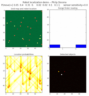
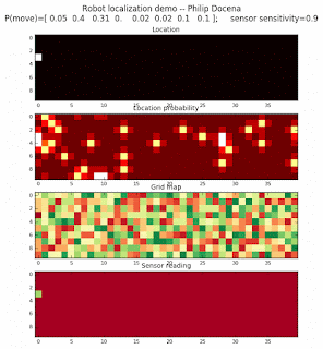
Below are an examples of how this could be done. The first graph is the location of the robot. The second is the current estimate of possible locations, shown as a heat map where high temperature (white-hot) means higher probability for that cell to be the robot location. The third graph is the environment, represented as a grid map of different colors. The fourth graph shows what the single sensor detects (the color of the current location). The fourth graph does not provide any X-Y coordinates to the localization algorithm. We just show the coordinates to help confirm that it matches the gridmap.

This example simulates a ‘robot’ that has wheels that are unreliable. For every movement, it could end up in different neighboring cell locations. It might not even move, or it might veer off, with different amounts of probability (which I assign pre-run). The robot's movement is randomly generated, with a bias towards continuing its current trajectory (not immediate backtracking, to make the localization faster). The variety of colors in the environment is also randomly generated, via a pre-run setting on color densities. The gridmap loops around itself in all directions, a common practice in simple simulations to minimize bounds checking code. This simplication sometimes prevents the algorithm from settling on a single stable localization.

The movement probabilities is given as P(move) in the graph, where the array P(move) is [current location; one cell forward; two cells forward; three cells forward; one cell forward, veer left; one cell forward, veer right; two cells forward, veer left; two cells forward, veer right].

We also model an imperfect color sensor. For these runs, we keep it as 0.9 --that is, for each color reading, it is 90% likely that the sensor detected the correct color, and a 10% likelihood that it failed and the cell is in fact a different color. Intuitively, we expect that the robot with an imperfect sensor will have a harder time finding itself accurately if neighboring cells have different colors. The worse the sensor, the harder the search.

The simulations below are limited to approximately 20 steps to minimize the GIF file size. Each step is made up of two sub-steps: a sensing step where the robot determines the color of its current grid cell, and a movement step where the robot moves based on a pre-generated random sequence. Notice that the probabilities become more precise with each color sensing step as the robot determines more exactly where it might be, and become less precise with each movement, because the robot has to assume multiple locations due to its 'faulty' wheels.

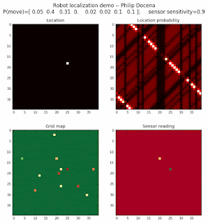
Demo 1A: box map, multi-directional movement, probabilistic motion, seed=0

The first demo allows the robot to move in any of four directions (left, right, up, down).

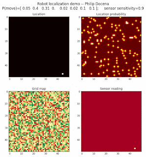
Demo 1B: box map, multi-directional movement, probabilistic motion, seed 1

The second demo is similar to the first, but with the robot following a different set of randomly generated movements.

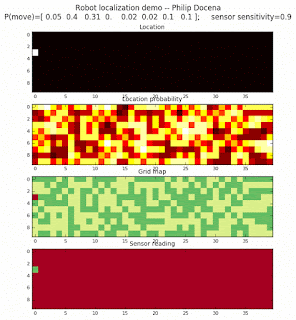
Demo 1C: rectangle map, left-to-right movement only, seed 0

The third demo below restricts the robot to move only from left-to-right.

Demo 1D: rectangle map, left-to-right movement only, seed 1

The fourth demo is similar to the third, but with a different initial robot location.


Localization theory

This is based on the Udacity/Georgia Tech lecture on localization (the Markov/discrete variety, the simplest kind of localization), under AI for Robotics taught by Prof. Sebastian Thrun. He is famous for Stanley, the Stanford-entered autonomous car that won the DARPA Grand Driving Challenge in 2005. Thrun went on to work on Google’s self-driving car effort. His work, along with those of competing teams, became the lynchpin for today’s autonomous driving cars.

The theory is actually as simple as we described it above. It is a series of measurements and updating probabilities until most locations are eliminated as unlikely. As the robot moves, we just spread out to its possible locations. As we stop and sense the color of the current grid, we then update probabilities, penalizing those that do not match and increasing those that do. In theory, the location estimates are adjusted based on pre-established movement probabilities. In other words, if a robot was given an order to move its motors, there is an assumption of its range of possible motion/translation in the real world. This could also be fully replaced by a step to read inertial sensors, then build the probabilities based on the empirical probabilities of these inertial sensors. In other words, it will just be a series of sensor readings: read color sensor, read inertial sensor, read color sensor, and so on, independent of the motor commands.

Experiments with more precision

With better mechanicals and motion controls, we can make the robot movement more precise. In our simulation, let’s presume that we now have a robot that perfectly goes straight (no left-right deviations), but still has some errors with random wheel slippage. We can model this below. Notice that the spread of probabilities on each motion step is now purely along the axis of motion. We expect that we can find the robot more quickly than in the above example, and we do. It might be a little bit difficult to notice the color contrasts on the heatmap, but the algorithm can in fact calculate the location probabilities more precisely at each step.

The simulations below were done on exactly the same settings as those above, except for the P(move) probabilities, as shown in the graph title. We still have motion unreliability, but we restrict it to 0-3 cells directly in front of the robot.

Demo 2A: no side slip, box map, multi-directional movement, seed 0

Demo 2B: no side slip, rectangle map, left-to-right movement only, seed 0

Demo 2C: no side slip, small map A, left-to-right movement only, seed 0

Demo 2D: no side slip, small map B, left-to-right movement only, seed 0


This could be easily adopted –or rather I am very curious if it could be adopted easily-- to actual robots running over colored tiles, i.e., LEGO Mindstorms, which I will leave as a future project. We can also appreciate that this can be easily scaled to more sophisticated sensors and maps, e.g., a simple non-GPS drone navigation system using a local overhead map, and the sensor probabilities can be based on matching map features taken by a drone camera.

Closing thoughts

With the demo code that generated the above demo animation, I tested and produced interesting results on the accuracy tradeoffs between the two sensor probabilities (the color detector vs. the motion detector), and how the localization prediction behaves under different color densities and number of colors. We will not explore these results here as there are more interesting things to pursue on discrete localization.

Wednesday, May 17, 2017

Hiding an image using Linear Algebra

Hidden image


Hiding and recovering an image using Linear Algebra

(This is a continuation of the previous post on morphing images (here). Since the concepts and code presented here build on the previous code, it is highly recommended to view the previous post first.)

In the previous post where we morphed one image into another, it was visually noticeable that during the transition, the two original images were discernable at the same time. In other words, the morphing process retained information for both images as one image dissolved while the other faded in. The image that is fading out was effectively being hidden away as we saw more of the new image.

The obvious question then arises: given the new image and the morphing process, can we recover the hidden image fully? Let's figure this out.

Back to linear algebra

If we think about the difference vector between the two images and the general parametric equation of a line, we might notice that for the equation of the line running along the vector direction, the length of the difference vector is irrelevant.

$$\begin{align}\ell_3 &=\{\mathbf v_1 + t*(\mathbf v_2-\mathbf v_1)\,:\, t \in \mathbb R \}\\ &=\{\mathbf v_2 + t*(\mathbf v_1-\mathbf v_2)\,:\, t \in \mathbb R \}\end{align}$$

We could have a shorter (or longer) vector $\mathbf v_3^{'}$ (whereas $\mathbf v_3=\mathbf v_2-\mathbf v_1$), yet we would always find the correct vector length for $t*\mathbf v^{'}_3$ to get to $\mathbf v_2$ exactly, by searching for just the right value of the scalar $t$. This is the same intuition we could use to recover another image along the difference vector (in fact, any image along the line that runs through this vector, even those outside the vector itself).

We therefore need two points along the difference vector to form a shorter vector. We could select any two points, but we will pick the last two images in the morphing sequence so the images will look similar. We can then calculate a scalar that would bring us to the other image exactly, recreating that other image. And then we are done.

So, let's write the code. This would be mostly similar to the previous code.

In [1]:
# import libraries
%matplotlib inline
import numpy as np
import matplotlib.pyplot as plt
#from scipy import misc
from PIL import Image

def get_image(fname):
    im=Image.open(fname)
    y,x=im.size
    img_dim=(x,y)
    img=np.array(im)
    
    # convert RGB to grayscale
    r,g,b=img[:,:,0],img[:,:,1],img[:,:,2]
    img=0.2989*r+0.5870*g+0.1140*b
    
    img=np.abs(img-255)  # invert colors
    img=img.flatten()    # flatten arrays
    
    return img,img_dim

img1,im_dim=get_image('img_A.jpg')
img2,_=get_image('img_B.jpg')


With pictures of happy people loaded (copyright reserved :) ), let's display the sequence of morphed images, just like in the previous post.

In [2]:
def display_vector(img,im_dim,pix_size=1):
    plt.figure(figsize=(img.shape[0]*pix_size,img.shape[0]*pix_size))
    for i,im in enumerate(img):
        ax=plt.subplot(1,len(img),i+1)
        #ax.set_title(img)
        ax.set_axis_off()
        a=np.reshape(im,(im_dim))
        ax.imshow(a,cmap='Greys',interpolation='nearest')
    plt.show()
    
# build a line segment/set of 'point images' via a parameterized line equation
img3_set=np.array([img1+t*(img2-img1) for t in np.linspace(0,1,num=11,endpoint=True)])
display_vector(img3_set,im_dim)


The idea is to generate the equation of the line $\ell_3$ by using two of these images. This gives us the correct vector direction to get to $\mathbf v_1$. We then extrapolate by scaling $\ell_3$ to get to $\mathbf v_1$ exactly, in theory anyway.

To show that we are indeed going to recover the first image, without using its existing loaded copy, we should delete it.

In [3]:
# delete img1 and check references
print('Deleting img1...')
del img1
print('Printing img1... (an ERROR message line will print if there is an error.)')
try:
    print(img1.shape)
except Exception as e:
    print('ERROR:',e)
Deleting img1...
Printing img1... (an ERROR message line will print if there is an error.)
ERROR: name 'img1' is not defined


Now we are sure that there is no trace of the first image.

Next, let us try to recover it. Since we generated 11 images while morphing, we can use the 11th image (which is the second of the source images, the target of the morphing), and the 10th image in the sequence (the last morphed image). We want the closest neighbors possible so the images would look alike naturally and would not show a superimposed outline of the image we are trying to recover.

To recover the first image in the morphing sequence (which is the first of the source images, the starting point of the morphing), we need to calculate $t$. This is simply $t=10$.

In [4]:
# reconstruct img1 from img2 and a member of img3
img4=np.array([img2+10*(img3_set[9]-img2)])
display_vector(np.array([img2,img3_set[9],img4]),im_dim,pix_size=4)


So there. We recovered the first image. We extracted a relatively clean image from a grainy source. We can prove this also at the pixel level by comparing the two images.

In [5]:
img1,_=get_image('img_A.jpg')
img_delta=img1-img4
print('Difference of the two image vectors:',img_delta)
print('Count of non-zeroes, threshold of 1e-5:',np.sum(img_delta>1e-5))
Difference of the two image vectors: [[  0.00000000e+00   2.84217094e-14   8.52651283e-14 ...,   8.52651283e-14
   -8.52651283e-14   8.52651283e-14]]
Count of non-zeroes, threshold of 1e-5: 0


The above result proves that the two images are approximately equal. The insignificant differences are due to computational limits.

Let's see if we can do the opposite, that is, recover a grainy image from a clean source. We know this is possible --the math is exactly the same-- but I want to show a side effect that is not obvious above because of the grainy source image.

In [6]:
img1,_=get_image('img_B.jpg')
img2,_=get_image('img_A.jpg')

# build a line segment/set of 'point images' via a parameterized line equation
img3_set=np.array([img1+t*(img2-img1) for t in np.linspace(0,1,num=11,endpoint=True)])
display_vector(img3_set,im_dim)

# delete img1 and check references
print('Deleting img1...')
del img1
print('Printing img1... (an ERROR message line will print if there is an error.)')
try:
    print(img1.shape)
except Exception as e:
    print('ERROR:',e)

# reconstruct img1 from img2 and a member of img3
img4=np.array([img2+10*(img3_set[9]-img2)])
display_vector(np.array([img2,img3_set[9],img4]),im_dim,pix_size=4)
Deleting img1...
Printing img1... (an ERROR message line will print if there is an error.)
ERROR: name 'img1' is not defined

We recovered the first image, but the middle picture is obviously fake, with apparition-like artifacts from the first image superimposed (hard to see at this resolution, but we can still see the Batman cowl over the headboard). Can we avoid this?

Sure, we can. We simply create a shorter line segment. We can do that by morphing with more images, so the penultimate image in the morphing sequence will be very similar to the source image.

Let's try it below. We will not show the intervening morphed images since we plan to create a lot. [On second thought, we do not have to create all the interim morph images. We just need the last morph.]

In [7]:
img1,_=get_image('img_B.jpg')

# build a line segment/set of 'point images' via a parameterized line equation
#img3_set=np.array([img1+t*(img2-img1) for t in np.linspace(0,1,num=101,endpoint=True)])
#display_vector(img3_set,im_dim)

# we do not need to create the whole set, just the penultimate member of the set
print(np.linspace(0,1,num=101,endpoint=True))
img3_set=img1+0.99*(img2-img1)
[ 0.    0.01  0.02  0.03  0.04  0.05  0.06  0.07  0.08  0.09  0.1   0.11
  0.12  0.13  0.14  0.15  0.16  0.17  0.18  0.19  0.2   0.21  0.22  0.23
  0.24  0.25  0.26  0.27  0.28  0.29  0.3   0.31  0.32  0.33  0.34  0.35
  0.36  0.37  0.38  0.39  0.4   0.41  0.42  0.43  0.44  0.45  0.46  0.47
  0.48  0.49  0.5   0.51  0.52  0.53  0.54  0.55  0.56  0.57  0.58  0.59
  0.6   0.61  0.62  0.63  0.64  0.65  0.66  0.67  0.68  0.69  0.7   0.71
  0.72  0.73  0.74  0.75  0.76  0.77  0.78  0.79  0.8   0.81  0.82  0.83
  0.84  0.85  0.86  0.87  0.88  0.89  0.9   0.91  0.92  0.93  0.94  0.95
  0.96  0.97  0.98  0.99  1.  ]


We delete the first image once again.

In [8]:
# delete img1 and check references
print('Deleting img1...')
del img1
print('Printing img1... (an ERROR message line will print if there is an error.)')
try:
    print(img1.shape)
except Exception as e:
    print('ERROR:',e)
Deleting img1...
Printing img1... (an ERROR message line will print if there is an error.)
ERROR: name 'img1' is not defined


Then we re-construct the little dude in the Batman costume (and quite frankly, he needs to adjust the cowl if he wants to successfully find baddies, fight crime and deliver the hammers of justice).

In [9]:
# reconstruct img1 from img2 and a member of img3
img4=np.array([img2+100*(img3_set-img2)])
display_vector(np.array([img2,img3_set,img4]),im_dim,pix_size=4)

Success! As you will notice, the second image no longer shows the ghostly apparition of Kid Batman.

How can we use this to hide images?

Consider two persons, Person A and Person B. Person A sends Person B image #1. Person B wants to send image #2 to Person A discreetly. Person B hides image #2 inside image #1, creating image #3. Person B sends image #3 to Person A, along with the number to recover image #2 via a separate channel. This number could perhaps also be embedded inside image #3. Person A can then easily extract image #2.

But we have to consider one more problem. We demonstrated a recovery sequence that uses the same full image array throughout, without saving and loading from an image file in the interim. The communications scenario described above will require the Numpy arrays to be saved into an image file before being sent across. Most files are created based on lossy compression algorithms, so the receiver might not be able to rebuild exactly the same full image array.

I am not sure about this assertion. I am unfamiliar with how image compression algorithms compress and extract images, and if different variants/versions of the same decoders produce different extracts from the same file, even if by only a few pixels, or if different compression algorithms ultimately create the same image array. For example, in the array->jpeg->array->png->array sequence, would the first and last arrays similar? I leave this to readers. These differences, if any, would cause distortions in the recovery portion, which might compound underflow/overflow risks.


Numerical stability

Basing the recovery on a morphed image that is only very slightly shifted might create some problems, if the difference becomes too small. As the vector difference becomes small, computational limits might cause accumulate rounding discrepancies (underflow/overflow) where the resulting vector $\mathbf v_3$ will not exactly reach $\mathbf v_2$. For instance, if two pixels are different by 100, dividing into 100 morphs would mean a gradual increase of 1 each time. But this might cause other pixels to increase by less than 1.0 each time, and integer rounding (RGB and grayscale are integers from 0 to 255) might cause some instabilities. We have even seen small differences even with just 10 morphed images, so 100 would definitely veer farther from $\mathbf v_2$. For simple purposes, as we did here, this is not a big concern.