Localization over heterogeneous features, part 1

Localization under different environments

In the previous post (here), we introduced a simple demonstration for discrete localization. Some of the examples did not clearly pinpoint a single location for the robot after the first 20 steps, although it did eliminate some locations as highly unlikely. With more iterations, the algorithm should be able to narrow down the possible locations to a few coordinates, perhaps even the actual robot location. Most of the incorrect location guesses were due to the imperfect sensor readings and the unreliable robot motion, modeled as probabilistic locations for each intended movement. In this post, we will evaluate if there are environments where the localization is faster.

The effect of environmental features diversity

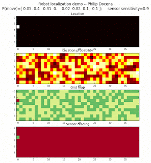
In the previous experiments, a major cause for the slower localization was the limited number of distinct environmental features. We used a fairly uniform densities for only three types of observations, i.e., three different colors over the gridmap. It is therefore easy to mistake one location for another given a color reading, even after matching a chain of color readings. In some cases, even when the intervening step(s) decreased the probability of a wrong candidate location, the next step would increase the probabilities again --while the probabilistic movements made the correct candidate location less precise. This caused the localization to linger over incorrect locations for a few steps.

Simulating the effects of environmental features diversity

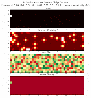
In this post, we explore if our hunch is correct: that an environment filled with more disparate features will allow a robot to localize quickly. Intuitively, this should be the case. A diverse environment allows a single observation to eliminate more candidate locations than would be possible in a more homogenous environment. In our simulation, if each cell was a different color, then a color reading would eliminate all but one cell, even with noisy robot motion, leading us to the correct cell location. If the color sensor is imprecise, the correct cell would still rise above its incorrect neighbors in a few steps.

We will model several environments using the same algorithm used in the previous post. We will vary the number of distinct features from 2, 4, 8, and 16. We can see the effect of these settings in the colors displayed on the grid map.

Demo 1a, all directions allowed, number of distinct features: 2

Demo 1b, all directions allowed, number of distinct features: 4

Demo 1c, all directions allowed, number of distinct features: 8

Demo 1d, all directions allowed, number of distinct features: 16

Let's also run several simulations on a left-to-right motion, as comparison to the previous post's experiments. We will also vary the diversity of features.

Demo 2a, left-to-right only, number of distinct features: 2

Demo 2b, left-to-right only, number of distinct features: 4

Demo 2c, left-to-right only, number of distinct features: 8

Demo 2d, left-to-right only, number of distinct features: 16

Closing thoughts

With these experiments, we established that the discrete localization algorithm can localize more quickly when the environment is more heterogenous. This also suggests that sensors that can detect different features are more useful in localizing than less discerning sensors, even when the latter are more accurate.

There are other experiments to explore. For example, does noisy motion affect localization in a diverse environment? In initial tests, in a highly chaotic map with small islands of cells (one or a couple of pixels) of the same color, a noisy motion leads to a harder time localizing, since practically any color could be reached in each step, so every cell tend to have some non-trivial probability. We will not explore this in detail at this time.

We could also model clusters of colors to reflect imprecise maps. In human terms, when we are inside a room, we can estimate that we are closer to one wall vs an opposing wall, but we would have to estimate if we are one fourth of the way, but would not know exactly (and we could be one-third or one-fifth closer to the wall). We can model this with color clusters in our map. Our intuition is that the probability will spread out across these clusters, but becoming more accurate as the robot detects a color change when traversing a cell cluster border. This is similar to being lost at sea without visible landmarks, but at least knowing you are in one of several island in the area when you get to any shore. This is indeed the case in initial experiments, which we will not pursue in more detail at this time.