Showing posts with label machine learning. Show all posts

Saturday, May 14, 2016

Perceptron, Part 2: How good is a model?

PLA_part_2

How good is a model?

In Part 1 of this series, we described the fundamentals of a perceptron and ran basic experiments. Now that we have a perceptron, we can address the logical next step.

How would an ML algorithm perform against data the model has not seen?

The answer is, we won't know until we run the model against actual test data that were not used to train the model, i.e., not in the training dataset. We would hope that the training data was representative of the test data so the accuracy would be similar. Given how the perceptron was guessing a solution, the final line was clearly one of many possible lines that could separate the two groups within the training dataset. As such, we expect a slightly lower accuracy on data that are not part of the training set. Based on the plots in Part 1, we knew accuracy would be off because we could see that the original separating line (the red line, the line that divided the training data set) and the final 'guess' line were not on the exact same location and orientation. Recall that the perceptron did not know the location of the red line. All it did was find a line that separated the data points it could see! Sometimes it was close to the red line; at other times it was a little off.

Let us now explore the intuition around potential error on new data, using trial runs and diagrams. The good thing is that we can easily modify the perceptron from Part 1 to run new experiments.

Learning curve: Tracking model accuracy

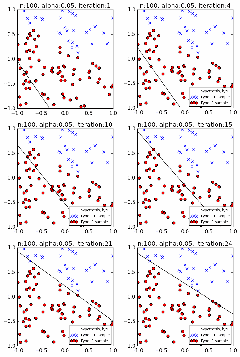
It was visually obvious from the different graphs in Part 1 that the more training samples used, the better the guessed line due to more training data points restricting the possible final guesses.

But what is 'better'? One simple method is by calculating the percentage of points correctly classified by a model. For a perceptron, it should reach 100% accuracy on a linearly separable training data set. The accuracy would tend to go up after every correction. To visualize this, we will graph the level of accuracy against the number of updates to the parameters of the separating line $\mathbf w$. In ML, each update iteration is commonly called an epoch. The resulting plot is called a learning curve. The curve would typically be rising, increasing accuracy with more training. However, since models are typically compared based on their errors on a given dataset, most ML learning curves track the error percentage instead. It is also typical to see a learning curve plotted against the number of training data points, instead of the epochs.

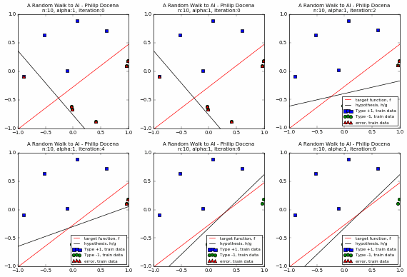
Let us look at a few simple runs with $n=10$ and $\alpha=\{1, 0.1, 0.05\}$, using two runs of each $n$ and $\alpha$ pair. Note that the iteration does not start with zero accuracy. The initial random guess line might already classify some points correctly; it might even be outside the plot window. Also, the plot-curve GIF pairs might be loaded at different speeds, and become out-of-synch unfortunately. This can sometimes be remedied with a page refresh, which forces a reload of temporary local copies of the GIFs:


Training set accuracy vs training repetitions

Let us compare the accuracy of a perceptron on the training dataset against training repetition. If a perceptron is 'learning', we expect its accuracy to improve with more iteration. This is indeed generally the case. The accuracy generally increases with each iteration. This is clear in the diagrams above. Generally, because in some cases, when the update 'overshoots', the PLA ends up with a momentarily worse accuracy. These tend to happen with higher learning rates, e.g., $\alpha=1$, as we expected from Part 1.

If we take learning rate as a proxy for the number of training repetition, since a small learning rate means small update steps, we can ask the following: does the learning rate have an effect on accuracy? We hold the number of training data points $n=20$ ($n=10$ is often too sparse) and vary the learning rate $\alpha$. Further, since we are tracking learning progress per iteration, we could ask an expanded question: does the learning rate have an effect on final accuracy, speed to reaching that final accuracy, and interim accuracy patterns?

We know that the PLA will always converge when run on linearly separable data, which is always the case in our data generator from Part 1 of this series. So the final accuracy is never in doubt. Any perceptron will have 100% accuracy over our randomly generated training data. Evaluating if intermediate accuracy levels rise faster under certain learning rates is a bit meaningless, however, because we always want to iterate as long as it reasonably takes to find a good accuracy rate. However, if there is a legitimate need to stop earlier (e.g., perhaps on complex models where iterations take a long time and some good enough accuracy could be used to stop iterations), it is worth observing how learning rates affect how fast the accuracy improves.

We compare two trials below, $n=20$ and $\alpha=\{1.0, 0.1, 0.05\}$. For each $n$ and $\alpha$ pair, the first three plots are for the three values of $\alpha$ while the fourth plot compares the different learning curves, c1 through c3.

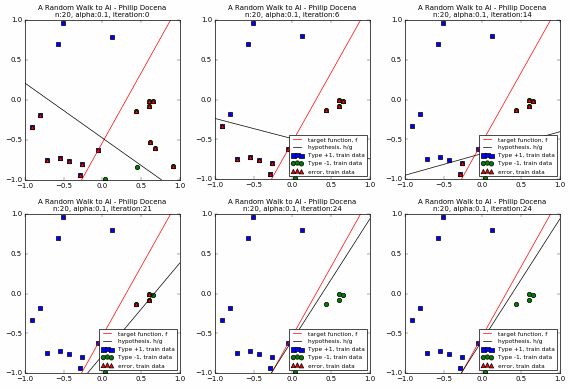

[A couple of runs did not reach 100% accuracy. This is an example where we force the PLA to stop. Recall in Part 1 that we explored the possibility of terminating the PLA before it finds a solution, either because there is no solution, or perhaps a run is taking a long time to converge. In this case, we stop for practical reasons: the PLA repeats only up to a maximum of ~35 iterations to control the size of the GIF file :). Typically, the perceptron used in our experiments converges at less than 50 iterations when $n << 100$, so ~35 iterations is often sufficient.]

Based on the above, we note that the choice of the learning rate $\alpha$ does seem to affect the speed to convergence. This was a point we loosely assumed in Part 1, but now we have learning curves to support that claim. The learning rate affects how 'noisy' is the march towards convergence. High learning rates tend to converge faster, simply because the 'guess' line is jumping around and 'chances' upon a solution quickly, whereas a low $\alpha$ crawls toward the solution.

But is that really the case? Did we just get lucky with the few samples drawn? How about if we increase the number of samples $n$? A high $\alpha$ run might move quickly in the beginning, but it could have difficulty settling into a final solution when there is little room for maneuvering around. Time for another experiment, $n=50$.


It turns out that there is no clear correlation between the learning rate and the speed of convergence. All we could see is that the high $\alpha$ scenario quickly moves closer to a solution but might have difficulty reaching a solution when there is a mix of data points near the dividing line (that is, a high number of training sample points), causing the PLA to overshoot and the learning curve to rise and fall repeatedly. In contrast, a low $\alpha$ run is slow to get near a solution, but its gradual movement is more assured of reaching a solution even in 'tight' margins. Its learning curve is gradually but predominantly rising, with few dips. In other words, in high $n$ runs, the higher $\alpha$ settings tend to take longer! This is at odds with our earlier findings at low $n$'s.

So maybe the trend depends on low or high $n$. Yet, that's also not assured. Contrary to this new trend during high $n=50$ trials, a low $\alpha$ run --such as the ($n=50$, $\alpha=0.05$) diagram-- could also take longer than a higher $\alpha=0.1$ run, even with high $n$! This happened because this run made slow progress in its early steps, and never caught up to the higher $\alpha$ models. Our findings appear to be that there is no clear pattern, and we might be better served if we focus on reaching the maximum accuracy possible (100% in our linearly separable data), with the number of training iterations a secondary consideration.

While both high and low learning rate models would have the same accuracy on the training data (100%, converged), against unseen data, it could be argued that a reasonably high (meaning, high but will converge) $\alpha$ will often be more accurate than a very low $\alpha$ run. This likelihood happens because, during training, a low $\alpha$ run would likely find a solution near the edges of the separation space/margin of the training set, whereas a high $\alpha$ run could jump into the middle of the same margin. More often, the border separating two classes of the testing set data is not at the margins imposed by the training set data. Hence, the high $\alpha$ has a higher likelihood of being more accurate. [We can test this --intuitively, this would be more obvious on models run on a small number of training data-- but for now we move on to another experiment.]

So instead we could ask: what if we hold the learning rate $\alpha$ constant while varying the number of training data points $n$ (not training iteration)? While this sounds like another good experiment, this would lead us into the same result: the accuracy would be 100% at some point, and it would just be a question of how long do we want the iterations to last, presumably faster with a smaller value of $n$ due to wide data margins. Perhaps a better question is: would the accuracy on previously unseen data be better with more training data, after allowing a perceptron to fully converge first on such training data? This sounds like another experiment. Our intuitive guess is yes (more data, better line estimate), but we might as well run some experiments anyway.

Training set accuracy vs testing set accuracy

We want to see if there is some trend between a training set accuracy and accuracy on data not used in training. In ML terms, the training set accuracy is called in-sample accuracy while the testing set accuracy is out-of-sample accuracy. Continuing on the above, we can run experiments where we fix $\alpha$ and vary $n$, but this time we will track both training data accuracy as well as test data (out-of-sample) accuracy.

We will reuse the previous code and add more data points that we will not use for training. We first create a large population of data points $N$, then we extract a small portion out of $N$ for use as our training data point $n$. We train on $n$, and test on $N-n$. We then track two learning curves, the in-sample and the out-of-sample curves. We will also plot the out-of-sample points and observe how the perceptron misclassifies certain out-of-sample points.

The changes to the Python data generator code are below. Adding these to the base perceptron code in Part 1 should be trivial.

In [ ]:
N = 500     # population
n = 10      # training sample size

# generate N random sample (population) using a uniform distribution from -1 to +1
P_N = np.array([np.random.uniform(-1, +1, N), np.random.uniform(-1, +1, N)])

# extract n points from population P as training points
X_n = np.array(P_N[:n, :n])

# determine the type of each point in sample X_n; false captures <=
type_mask = X_n[1] > slope * X_n[0] + b
type_mask_N = P_N[1] > slope * P_N[0] + b

# training data and population correct classification
y = [+1 if row == True else -1 for row in type_mask]
y_N = [+1 if row == True else -1 for row in type_mask_N]

# adjust vectors x in X_n and P_N to accommodate x_0
X = np.array(np.ones(shape = (n, d + 1)))
X[:,1:] = X_n.T
P = np.array(np.ones(shape = (N, d + 1)))
P[:,1:] = P_N.T

# initialize h for training set and h_N for entire population
h = np.array(np.sign(np.dot(w, X.T)))
h_N = np.array(np.sign(np.dot(w, P.T)))

# error masks and error curves
error_mask = h != y
error_mask_N = h_N != y_N
error_curve = []
error_curve_P = []

# out of error is entire population less in-sample
error_curve.append(1 - np.count_nonzero(error_mask) / np.size(error_mask))
error_curve_P.append(1 - ((np.count_nonzero(error_mask_N) - \
    np.count_nonzero(error_mask)) / \
    (np.size(error_mask_N) + np.size(error_mask))))

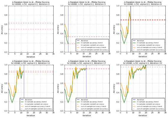
The plots of the different runs are below. Each run is presented via a pair of graphs: a scatter plot and a learning curve. The first group is from $n=50$, using two different learning rates each; the second group uses $n=10$.

This is similar to prior graphs, but let us look at the legends since this is now more cluttered.

The test data points are green 'x' and blue '+' dots. There are $N=10000$ of these points combined, out of which we extracted $n$ points. These became our training data points, but with the green 'x' changed to a circle and the blue '+' changed to a square. Misclassified training data points are labeled with a red upright triangle, while misclassified test data points are inverted yellow triangles (but seen as mostly black due to overcrowding). On the learning curves, we track two plots: the in-sample accuracy in green, and the out-of-sample accuracy in gold. The current accuracy of each curve is marked with dash lines.

Below are the runs for $n=50$.


Below are the runs for $n=10$. I further changed the colors to make identification easier. The training data points are now cyan squares (taken from the green x's) and orange circles (amid blue +'s). The misclassified test data points are now yellow tri-stars, avoiding the black outlines in the previous group. I then slowed the GIF for easier tracking.


A few more diagrams, conclusions, and next steps to follow

Monday, May 9, 2016

Perceptron, Part 1: How simple machines 'learn'?

PLA_part_1

Where do we start?


There are many ways to get started in machine learning (ML). Unfortunately, there are also a bewildering assortment of concepts and techniques. It is a little bit overwhelming. And the more one gets into ML, the more one realizes how much there is to know. Luckily, ML techniques tend to follow the same concepts, so understanding the common concepts would help frame other related algorithms. Let's explore some of the building blocks here.

How does a machine ‘learn’?


One of the easier ways to visualize how a machine learns from data is through a perceptron. Think of a perceptron as a mechanism that, after some trial-and-error, learns to automatically separate two sets of data. We give it a dataset containing two groups of something, and it will calculate a line that separates the two groups. The key part is that there is no explicit instruction provided (by humans) to calculate this line, other than a general instruction to minimize its mistake in classifying the items it is provided. Given a different set of the same two types of data, its learning progress will be different, but will generally be able to separate the two groups. Once a perceptron figures out this dividing line, it can then receive a new input, and it can decide whether that new input belongs to group A or group B. It is automatic, hence the learning part. Through some algorithm, it learns a pattern from the data, a pattern it uses to classify the data points into two groups.

The description above is intentionally vague. It might make more sense with some diagrams. The beauty with a perceptron is that its inner workings can be visualized as it goes through its trial-and-error phase.


This should give us an intuition on machine learning. But before we get there, let's wade through some math. :)

Perceptrons


After some fallow years in the 70s through the 90s (called the "AI winter"), AI has been in some renaissance, ML in particular. Using new techniques and clever rethinking of old techniques, AI and ML have been hogging headlines again in the last few years, the most recent was AlphaGo early this year. But perceptrons, one of the earliest machine learning techniques, are not new. They existed before "machine learning" was even part of statistics and computer science literature, let alone when ML entered the jargon of technology journalists. The basic idea was explored in 1943 by Pitts and McCulloch, and in 1958 by Rosenblatt.

Its mechanism is simple (although if you visit Wikipedia, depending on your background, it might seem hard to understand). Perceptrons are often covered in ML under neural networks --it is after all a mathematical representation of a (very simplified) neuron and is the simplest ML neural network-- but it can be studied without any knowledge of how neurons or neural networks work. Below is the core math that describes a perceptron and the perceptron learning algorithm (PLA). It might appear complicated. We will discuss these equations in the following sections, and include some actual Python code.

Note: I wrote the below based on how I understood the perceptron and its notations, so there is some likelihood my notation is a little different from a formal definition. Chances are the formal notation will be more compact (e.g., $\mathbf x \in \Bbb R^n$ and nothing else), leaving the intermediate constructs to the reader, based on familiarity with mathematical font styles and notations.

My goal was to de-construct this one, so I could more easily understand ML equations elsewhere. I am also only a couple of days into iPython Notebook and MathJax syntax, so I might have mislabeled some indices, superscripts, subscripts, or misused generally accepted font styles for certain variable types. I'll correct as I find errors. Writing accurate mathematical text is not easy! :)
$$\\ \\ y^{(i)} = \begin{cases} +1 & if \ f(\mathbf x^{(i)}) > threshold \\ -1 & otherwise \end{cases}$$$$\mathbf x^{(i)} \in \Bbb R^d,\;i=1,...,n$$
That is, $$\mathbf x^{(i)}=(x_1^{(i)},x_2^{(i)},...,x_d^{(i)})$$ $$\mathbf X=\{\mathbf x^{(1)},\mathbf x^{(2)},...,\mathbf x^{(n)}\}$$
The algorithm calculates, $h_\mathbf w(\mathbf x)$ as an estimate for $y$, $$h_\mathbf w(\mathbf x) \approx y$$ $$h_w^{(i)} = \begin{cases} +1 & if \sum_{j=1}^{d} w_j x^{(i)}_j > threshold \\ -1 & otherwise \end{cases}$$
by adjusting, $$\mathbf w \in \Bbb R^d$$ $$\mathbf w=(w_1, w_2,..., w_d)$$
We start with the following: $$\sum_{j=1}^{d} w_j x_j > threshold$$ $$\sum_{j=1}^{d} w_j x_j - threshold > 0$$
To simplify, we treat the activation threshold (also called bias) as a member of the summation, thus revising $\mathbf w$: $$\sum_{j=1}^{d} w_j x_j + w_0 x_0 > 0$$ $$\sum_{j=0}^{d} w_j x_j > 0$$ $$where\;x_0=1\; and \; \mathbf w \in \Bbb R^{d+1}\ ( \mathbf w=(w_0, w_1,..., w_d) ) $$ $$\bbox[yellow] {h^{(i)}_w(x)=sign(\sum_{j=0}^{d} w_j x^{(i)}_j)}$$
In vector notation: $$\bbox[yellow] {h^{(i)}_\mathbf w(\mathbf x)=sign(\mathbf w\bullet \mathbf x^{(i)})}$$ $$\bbox[yellow] {h^{(i)}_\mathbf w(\mathbf x)=sign(\mathbf w^T \mathbf x^{(i)})}$$
Given a set of training data $\mathcal D$, the PLA algorithm iteratively (the subscript $k$) calculates values for $\mathbf w$ until all data points $\mathbf x^{(i)}$ through $\mathbf x^{(n)}$ are correctly classified: $$\mathcal D=(\mathbf X, \mathbf y)=\{(\mathbf x^{(1)},y^{(1)}),(\mathbf x^{(2)},y^{(2)}),...,(\mathbf x^{(n)},y^{(n)})\}$$$$\bbox[yellow] {\; \mathbf w_{k+1}=\mathbf w_{k}+y^{(i)}\mathbf x^{(i)}\; }$$
ML is littered with mildly daunting math like these. And I made it more complicated by expanding the intermediate steps! The operations on each element in a vector, vs over entire vectors, become very confusing. However, with repetition, they start to look the same across different ML techniques and recognizable enough to skip some of the indices. There are some variations in notation, but the patterns are similar. The key is to keep track of the indices and font styles.

Indices everywhere!


We are tracking three indices: (i) the data point sample index $i$, (ii) the feature index $j$, and (iii) the code iteration index $k$.
  • The sample index runs from 1 through $n$ and is on the upper right corner of a variable $\mathbf x$, in a parenthesis, and only applies to $\mathbf x$. This can be disregarded or removed in a few places without changing the meaning. It is only there to remind me that this $\mathbf x$ is in fact one of many different $\mathbf x$'s.
  • The feature index runs from 0 (because of the adjustment above) through $d$ and is on the lower right corner of vector variables $\mathbf w$ and $\mathbf x$.
  • The code iteration index is $j$, ends where the code finds a solution or stops, and is on the lower left corner of variable $\mathbf w$.

Be aware though that often different indices are placed on the same corner, and it is up to the reader to determine what is referred via the font style. For example, instead of writing $x_i$ and $\mathbf x^i$, we might see $x_i$ and $\mathbf x_i$, with both indices on the lower right corner! It is implied however that the second $\mathbf x$ is a sample vector, not a vector element, so we would recognize it as referring to the sample index, not the feature index. Most equations will also keep on using $i$ for different indices, adding to confusion. Our only clue in this case would be the ending value: does it refer to features $d$ or sample $n$? Whew!!!

What do they mean?


Here's my attempt at explaining the above mathematical description:
  • $y$ is a variable, or a function, that can only take a value either -1 or +1. This is the target function, the function whose behavior we do not know and have to estimate. The -1 or +1 values indicate that this is a binary classifier (a data point will be identified as one type or another). The function $y$ outputs +1 if the value of the unknown function is greather than zero, -1 otherwise. For example, if we assume that this function represents a line (i.e., the dividing line described earlier), any point above this line is assigned the value of +1, else -1. To repeat, we do not know the exact formula for $y$, but we can estimate it by observing the points it generates.
  • $\mathbf x$, which appears in the function for $y=1$ and $h=1$, are the values of the features (read this as some measurable characteristics) associated with each data point. In a real example to identify a flower, we can think of one axis as representing the color of a flower, another axis as the average length of its petals, and so on. These can be any real number values (hence the set of real numbers $\Bbb R$). In our example below, we will limit the features from -1 to +1, and only use two features, thus two axes/dimensions: the horizontal axis feature, and the vertical axis feature. The number of features can be any number $d$. The 2-d representation will help easily visualize the dividing line. Each $\mathbf x$ (identified with the $i$ superscript) has its own features. We are given $n$ different data points.
  • $h(\mathbf x)$, our 'guess' for the line that divides the two sets of data. This may or may not be equal to $y$, but it would be close. The function $sign$ means it will output the sign of the enclosed calculation, in effect, -1,+1, or 0.
  • $\mathbf w$, which is also in the summation for $h=1$, is a set of parameters or weights. Its values affect the summation in $h(\mathbf x)$, hence it affects the location and orientation of the 'guess' line. They are automatically calculated by some algorithm. Each feature (axis) has its own $w$. This $w$ can be interpreted as controlling how much of the value of a feature is added to the sum (influences the line). For example, the algorithm might determine that to identify one flower vs another, it only needs to look at color, so color will have a higher weight effect than,say, petal length.
  • The summation of $w*x$ is an element-wise multiplication between corresponding $w$'s and $x$'s, followed by an addition --i.e., a sum of products. If we treat $w$ and $x$ as vectors (they are vectors, as $\mathbf w$ and $\mathbf x$), we can take advantage of vector operations. On a single example, we can use a dot product, which multiplies the transpose of $\mathbf w$ and $\mathbf x$, that is $\mathbf w^T \mathbf x$. There is no need to understand a transpose and a dot product for now (good internet references abound), as long as we accept that the result is the same as the sum of products.
  • The PLA is straightforward. It simply updates the values for $w$ (inside $\mathbf w$) whenever there is an error, and the magnitude of the change is equal to the value for $\mathbf x \bullet y(\mathbf x^{(i)})$. This will 'push' the value of $\mathbf w$ towards the opposite direction, exactly because whatever value of $h(\mathbf x_i)$ was generated by that $\mathbf w$, it led to an error. Therefore it has to be corrected, and $y(\mathbf x_i)$ is the opposite of $h(\mathbf x_i)$. Its influence (that is, the parameter weights $\mathbf w$) has to be lessened (or increased, depending on the sign of the correct outcome). $\mathbf w$ is a vector, so it is made up of $w_0$, $w_1$, and $w_2$. All of these will be updated. The larger the error in each feature ($x_0$, $x_1$, and $x_2$), respectively, the larger the correction for the corresponding $\mathbf w$ ($w_0$, $w_1$, and $w_2$).

Other important observations:
  • Target function $y$ vs guess function $h$: The rules that determine the value of $y$ in the above description is a function that depends on $\mathbf x$. It can be any function (but only linear functions can be cleanly separated by a PLA). In contrast, the estimate for $h$ has a more recognizable form --a linear equation, $h=w_0+w_1x_1+w_2x_2+...+w_dx_d$-- with parameter $w$. In our example later, we will pick a linear equation for $y$ using a similar form --$y=\beta_0+\beta_1x$, parameterized by $\beta$. In this context, the PLA is trying to find $w$'s that approximate $\beta$'s, as a way of approximating $y$. However, the formula for $y$ that generates the data points does not have to be in this form always, i.e., not $y = \beta_0 + \beta_1x$. As long as the data points generated by any form of $y$ and seen by the perceptron are separable, the PLA will find a line that separates these points, using a linear equation with parameter $\mathbf w$. We will explore an example later.
  • The update rule above, $\mathbf w_{i+1}=\mathbf w_{i}+y^{(i)}\mathbf x^{(i)}$ for a PLA, is common in ML. The more general notation is $$\mathbf w_{i+1}=\mathbf w_{i}-\alpha \delta \mathbf x^{(i)}$$ where $\alpha$ is the learning rate and $\delta$ is the error.
    • The learning rate is the size of the steps $(0 < \alpha \le 1)$ at which a learning algorithm 'learns'. Bigger typically means a faster path to a solution, but big steps can also mean a longer time to find a result because the PLA keeps on missing the solution by jumping too far, then jumping back too far again. If too large, the PLA might not even reach a solution. We will explore this via examples. The learning rate in PLA is generally set to 1.0. In ML notation, the learning rate is also represented as $\eta$.
    • The $\delta$ represents the magnitude of the error caused by the current guess, and its value is used to adjust the weight $w$. The bigger the error, the bigger the adjustment. In PLA, this is simply -1 or +1, the value of $y$. It could also be calculated as $-1*(h(x_i^{(i)}) - 0)$, but this fails when we initialize at $\mathbf w=\mathbf0$, or as an error term, $(h(x_i^{(i)}) - y(x_i))$. This latter version is used in a variation of a perceptron (called Adaline, for Adaptive Linear Element), and is a direct effect of the Adaline's use of $(h(x_i^{(i)}) - y(x_i))^2$ as its error measure, otherwise known as squared error. This is an error measure that will come up again, in linear regression for instance.

The Perceptron Learning Algorithm (PLA)


Let's parse the above mathematical description into code. The entries in yellow highlight above are what matters. $h_w(\mathbf x)$ is a 'guess' line. It may or may not be close to the 'actual' line $y$. The location and orientation of $h_w(\mathbf x)$ is influenced by parameters inside the current vector $\mathbf w$. The first three highlighted formula are similar, just different ways of representing $h_w(\mathbf x)$. The parameter vector $\mathbf w$ is updated using the fourth highlighted formula (this is the 'learning' part).

A little prologue on the code


I use Python. It is easy to learn and read. More importantly, I need Python because of little libraries that make programming ML algorithms easy. One such helper library is called NumPy. NumPy provides support to handle large, multi-dimensional arrays and matrices, along with fast mathematical operations commonly applied to arrays. Other useful libraries are: matplotlib (for plotting graphs), SciPy (a NumPy extension focused on scientific calculations), scikit-learn (a library of ready-made ML algorithms), and pandas (for extracting data from files).

The general logic of the perceptron learning algorithm is as follows:
  1. Start with a 'guess' line.
  2. Pick a point in the dataset. Calculate its type based on the guess line in #1. If it is to the left of the line, say, Type A; Type B otherwise.
  3. Check if the guessed type is correct. If misclassified, adjust the location/orientation of the 'guess' line so this particular point becomes correctly classified. This adjustment might mean the new 'guess' line will cause misclassifications elsewhere that would otherwise have been correct in the previously guessed line. This behavior of sometimes causing more misclassifications is to be expected.
  4. Repeat from #2 until all points are correctly classified, or the algorithm reaches a pre-defined stopping criteria.

Most PLA code will randomly select a misclassified point. In this code, I go through the points in sequence, checking if it is misclassified. The points are randomly generated at the start, so this shortcut does not affect the PLA search other than a slower execution, while allowing predictable/reproducible runs.

In Python, the core code is made up of the following lines:

In [ ]:
# this is a code fragment and won't run; merge with data generator to run
# this is meant to show the surprisingly short PLA logic

# setup parameters
d = 2       # number of features
rate = 0.1  # learning rate

# prepare weights vector w and feature vector X, including w0 and x0=1
w = np.random.rand(d + 1)
X = np.array(np.ones(shape = (n, d + 1)))
X[:, 1:] = X_n.T     # X_n is from the data generator, check dimensions

# initialize guesses vector given initial weights
h = np.array(np.sign(np.dot(w, X.T)))

# set error flag
error_mask = h != y
error = True if error_mask.any() else False

# while there are errors, keep on processing
while error:
    
    # sequentially go through data points
    for i, xn in enumerate(X):
        
        # calculate the type based on current weights
        h[i] = np.sign(np.dot(w.T, xn))
        
        # is guess the same as the actual type?
        if h[i] != y[i]:
            
            # update weights if error
            w += y[i] * xn * rate
            
            # update guesses vector given new weights
            h = np.array(np.sign(np.dot(w, X.T)))
            
            # check for remaining errors
            error_mask = h != y
    
    # check for remaining errors after for loop
    error_mask = h != y
    
    # update error flag
    error = True if error_mask.any() else False

Notice that the operations closely follow the mathematical description earlier. This is made possible by NumPy (NumPy has a sign function, who knew!?!). The one odd thing is that NumPy creates arrays as row vectors, so the transpose is not necessary (the transpose does not seem to have any effect against 1-d arrays). The only calculation not shown in the previous equations is applying $\mathbf w$ against the entire matrix of $\mathbf X$ (that is, all data points $\mathbf x^{(1)}$ through $\mathbf x^{(m)}$), which we need to quickly detect misclassified points. Several other options are provided below for comparison.

In [ ]:
# The following operations produce the same h[i].
# w and x are 1d arrays (row vectors) so the transpose has no effect.
# the first entry is the sum of products method
h[i]=np.sign(np.sum(w*xn))
h[i]=np.sign(np.dot(w,xn))
h[i]=np.sign(np.dot(xn,w))
h[i]=np.sign(np.dot(w.T,xn))
h[i]=np.sign(np.dot(w,xn.T))
h[i]=np.sign(np.dot(xn.T,w))
h[i]=np.sign(np.dot(xn,w.T))
h[i]=np.sign(np.dot(w.T,xn.T))
h[i]=np.sign(np.dot(xn.T,w.T))

# The following operations produce the same h.
# w is a 1d array (row vector) so the transpose has no effect.
# X, a matrix, has to be transposed if second argument in numpy.dot().
h=np.array(np.sign(np.sum(w*X,axis=1)))
h=np.array(np.sign(np.dot(X,w)))
h=np.array(np.sign(np.dot(X,w.T)))
h=np.array(np.sign(np.dot(w,X.T)))
h=np.array(np.sign(np.dot(w.T,X.T)))

Why is NumPy useful in ML code?


NumPy allows vectorized array operations. Most operations in ML use vectors, which are typically represented as arrays in code. In standard programming, if we have to add elements of two arrays, we will write for loops for each axis, then add each element. It is easy to make a mistake in the indices of these loops and arrays. For loops in Python are also slow. Vectorized operations are far simpler: we just add two vectors like we would add two simple variables. NumPy does the hard work. And they are a lot faster! Pure Python code is slow, whereas NumPy uses optimized C libraries perfected by an army of highly motivated expert volunteers. The examples below produce the same result: (i) a traditional for loop, (ii) a Python list comprehension, and (iii) vector addition, with broadcasting. List comprehensions are typically faster than for loops, but in this example, this method creates different arrays inside the list comprehension itself, which renders the list comprehension pointless. Notice the runtimes....
In [1]:
import numpy as np
import timeit

# use traditional nested for loops
def forloop(go_print):
    for i, b_row in enumerate(B):
        for j, b_rowcol in enumerate(b_row):
            # add, element-wise, A to each row in B
            C[i,j] = A[j] + B[i,j]
    if go_print: print('C = A + B, using nested for loops:', C)

# use Python's list comprehension
def listcomp(go_print):
    C = np.array([[a_rc + b_rc for a_rc, b_rc in zip(A, b_row)] for b_row in B])
    if go_print: print('C = A + B, using nested list comprehensions:', C)

# use vectorized addition
# NumPy will 'repeat' A to match the number of rows in B; 'broadcasting' in NumPy
def vector(go_print):
    C = A + B
    if go_print: print('C = A + B, using vectorized addition:', C)

# main code
# generate some arrays
A = np.ones(3)
B = np.array([(2,2,2),(3,3,3),(4,4,4)])
C = np.zeros(shape=(3,3))

print('A:', A)
print('B:', B)

# print results
forloop(True)
%timeit forloop(False)
listcomp(True)
%timeit listcomp(False)
vector(True)
%timeit vector(False)
A: [ 1.  1.  1.]
B: [[2 2 2]
 [3 3 3]
 [4 4 4]]
C = A + B, using nested for loops: [[ 3.  3.  3.]
 [ 4.  4.  4.]
 [ 5.  5.  5.]]
100000 loops, best of 3: 9.6 s per loop
C = A + B, using nested list comprehensions: [[ 3.  3.  3.]
 [ 4.  4.  4.]
 [ 5.  5.  5.]]
100000 loops, best of 3: 10.1 s per loop
C = A + B, using vectorized addition: [[ 3.  3.  3.]
 [ 4.  4.  4.]
 [ 5.  5.  5.]]
The slowest run took 6.06 times longer than the fastest. This could mean that an intermediate result is being cached.
1000000 loops, best of 3: 1.41 s per loop

The rest of the code are to create the data and plot the graphs. It took me a lot longer tweaking the sample data creation (Numpy random) and graphs (matplotlib) than coding the PLA section. This was both a satisfying and a frustrating point: writing ML-specific code is not that bad after all is said and done, for a perceptron anyway, but refining the graphics and presentation takes a lot more trial and error!

Data generator


The data generator creates a vector of 2-d points over a sample space from -1 to +1 in each axis, using a uniform random number generator. Then it generates two (x, y) points to mark the end points of a line. This is the separation line. On one side of this line, all sample points are labeled as Type +1. On the other side are Type -1, including points that happen to be exactly on the dividing line. We can also run a model that assigns 0 to points that are collinear to the dividing line. For simplicity here, there is no Type 0 on the training data labels. The PLA code with numpy.sign() just assumes a 0 is a mismatch.

In [1]:
import numpy as np
import matplotlib.pyplot as plt

# setup sample size and dimensions (fixed at 2d)
d = 2         # features, dimensions
n = 10        # sample size
# generate n random sample using a uniform distribution from -1 to +1
X_n = np.array([np.random.uniform(-1, +1, n), np.random.uniform(-1, +1, n)])
print('X_n:', X_n)

# generate the two end points of the separating line
x_div = np.array([np.random.uniform(-1, +1), np.random.uniform(-1, +1)])
y_div = np.array([np.random.uniform(-1, +1), np.random.uniform(-1, +1)])
print('x_div:', x_div)
print('y_div:', y_div)

# slope and y-int calcs from m=rise/run and y=mx+b
# slope will fail on divide by zero, so just restart if error
slope = (y_div[1] - y_div[0]) / (x_div[1] - x_div[0])
b = y_div[0] - slope * x_div[0]
print('slope:', slope)
print('b:', b)

# determine the type of each point in sample n; false captures <=
# the mask is useful in plotting points; otherwise, calculate y directly
type_mask = X_n[1] > slope * X_n[0] + b
print('type_mask:', type_mask)

# training data correct classification;  calculate y for each data point
y = [+1 if row == True else -1 for row in type_mask]
print('y:', y)
X_n: [[-0.76631334 -0.68215067  0.54632103  0.36858243  0.90957209  0.78716714
   0.69118626 -0.40030246 -0.30352267 -0.9326125 ]
 [-0.95160552 -0.03176065 -0.96411528 -0.782851    0.26217029 -0.87982399
  -0.7449728  -0.32062671  0.07532858 -0.26872037]]
x_div: [-0.15960529  0.75742281]
y_div: [ 0.08988555 -0.34202446]
slope: -0.470988856542
b: 0.0147132394822
type_mask: [False False False False  True False False False False False]
y: [-1, -1, -1, -1, 1, -1, -1, -1, -1, -1]


Plots of initial trials


Let's test the code. The PLA is trying to find a line that separates the two groups of data (blue circles and green squares). This guessed line might not be the exact line that we used to assign points to a group (the red line), but it will be close. The PLA does not know the location of the red line. Getting as close to this original line using only a small set of observations is the whole point of ML.

The images are faster than the actual code. The images capture the iterations when there is an update to $\mathbf w$, that is, when there is a discrepancy, whereas the actual code goes through all points sequentially. The progress of the actual code slows down as it gets closer to a solution, because almost all of the points have been correctly classified at that point.

These examples use $n=10$ samples, and a learning rate $\alpha=0.1$. The small learning rate shows a gradual shift towards the red line, whereas $\alpha=1.0$ will cause huge and seemingly random jumps.


Below are $n=50$ examples. Note the higher accuracy (closer to matching the red line) with more n samples, and the longer iteration. Even with a small learning rate, when there is a very thin gap between two opposing points relative to the orientation of the current best line, the PLA tends to overshoot:


Wait, this thing is guessing each time?
You're right. But it is guessing with some 'intelligence' built-in. It is using the error to make adjustments. It gets better each time (it can also get worse sometimes), but over many iterations, it is more likely to get better. In fact, in a PLA with a low learning rate and linearly separable data, it will converge to a solution.

... this sounds like something in calculus.
Yes and no.

Yes, this is similar to minimizing some function, which is the magnitude of the discrepancy between the guessed type relative to the actual type of a data point.

No, because a PLA does not strictly apply an error value as the adjustment. It simply forces either a -1 or a +1 multiplier as the error adjustment. In fact, trying to minimize $h(x)$ for a PLA using a single expression is considered impossible because it is a step function (jumps abruptly from -1 to +1).

If this were an Adaline network, where the adjustment is $(h_x-y)\mathbf x$, then the algorithm is minimizing some function exactly the way we do in calculus, and is an example of stochastic gradient descent. We will encounter this term many times in ML. For now, think of it as a way to find the lowest value of some error function.


Now that we know how it works, let's answer a few easy questions


-- Does it matter where you start the line (i.e., initial conditions)?
No, the update will start to move the line to the intended target.

-- What happens if we tweak some of the PLA parameters?
We did a few tweaks above, by changing the number of training data $n$ and the learning rate $\alpha$. A higher $n$ helps accuracy, but tends to take longer. A lower $\alpha$ slows progress, but the march to the solution is more certain.

-- What happens if the scales are not equal?
The bigger scaled axis will dominate the update, and the iteration will take longer as it will tend to converge on the dominating axis first. The iteration will generally take longer. We can test this easily.

-- What happens if the range is 0-1, not -1 to +1?
It should still work. The value of $\mathbf x$ is part of the update. This is also easy to test.

-- Will it always find a line that cleanly separates the sample data?
If the data available for training is separable by a straight line, yes. The more precise answer is yes, if the data points used in the training are separable by a straight line. That is, we can manipulate and transform the original points into a different set of points that can then be separated by a straight line. This is an advanced concept that we will not cover here (maybe in a future post). This often involves adding more features/axes, some might be new features (more data!), or some could be composites or transformations of existing features. The thinking is that the new representation would show that the two groups are linearly distinct from each other. However, finding actual fully linearly separable data is rare. We often have to assume a level of misclassification.

-- If the target function $y$ is not known, how do we know that it is linearly separable?
We won't know. The PLA will only converge (stop) if the sample generated by $y$ and given to us for training purposes is linearly separable. If not linearly separable, the PLA will not stop.

-- There should be a mechanism to stop, if the search is not working out!
There should be. To force a PLA to stop, we can either stop by setting a maximum repetition threshold (e.g., run 200 times max), or by setting an acceptable accuracy/error threshold (e.g., stop if less than 2% of data points are misclassified).

-- But if it stops suddenly, and because the 'guessed' line appears to be jumping around while the PLA is searching, wouldn't we end up with a worse 'guessed' line if we stop at the wrong time? In this case, can't we go back to an earlier better line? Sounds like a logical thing to do.
Yes, this is called the Pocket algorithm. Before I learned that it had an official name, I called it king-of-the-hill, a standard algorithm useful when sequentially searching for max/min over a list. As we go through a list, we keep the best so far, replacing only when we find a better choice. Changing the above code to accommodate the Pocket algorithm is a trivial change. We do have to create a measurement for what is 'better', such as the percent accuracy.

-- How can we ensure that the guessed line is close enough/as close as possible to the actual line that separated the data?
This is the question. And this is exactly what scientists and researchers are trying to improve: getting as close as possible to an unknown line, given a limited set of training data. The non-answer answer is: there are different techniques out there. And like you, I am excited to learn them....


How does this connect to other ML techniques?


The perceptron is a binary linear classifier. From here, we can go to linear regression (conceptually similar to a perceptron, except it produces real numbers instead of +1/-1), logistic regression (a linear regression with real number output restricted to between -1 and +1), neural networks (a perceptron is in fact a very simple neural network), and support vector machines.

Can we see this in action using real data?


We will try a little experiment in the future, using standard 'toy' datasets commonly used in ML.

Next stop: More PLA experiments


Now that we have the foundations for a linear classifier, we can test various scenarios to see how ML learning behaves, in the context of a perceptron.